Machine learning has become quite successful in several domains in the past decade. An important portion of this success can be associated to the availability of large amounts of data. However, collecting and labeling data can be costly and time-consuming in many fields such as speech recognition, text classification, image recognition, as well as in robotics. In addition to lack of labeled data, robot learning has a few other challenges that makes it particularly difficult:
- Learning from demonstrations has recently been popular for many tasks. However, we cannot just rely on collecting demonstrations from humans to learn the desired behavior of a robot, since human experts usually provide suboptimal demonstrations or have difficulty operating a robot with more than a few degrees of freedom. Imagine you are to control a drone. Even if you are an expert on it, how optimal can you be on completing a task, e.g. following a specific trajectory as quickly as possible?
- We could just use reinforcement learning to have the robot optimize for itself, but what will be the reward function? Beyond cases where it is easy to automatically measure success or failure, it is not just hard to come up with an analytical reward function, but it is also hard to have humans assign reward values on what robots do. Imagine you are watching a robot grasping an object. Could you reliably answer if you were asked: “On a scale of 0 to 10, how good was that?”. Even if you can answer, how precise can you be?
- Both demonstrations and human reward labeling have another shared problem: scaling. Given that most supervised learning and reinforcement learning techniques need tons of data, it would take humans giving demonstrations or labeling rewards for years and years just to train one agent. This is clearly not practical.
So what can we do? One alternative is preference-based methods - instead of asking users to assign reward values, we will show them two options and ask them which one they would prefer. Furthermore, we are going to use active learning techniques to have the robot itself ask for queries that would give the much information. While the use of active learning helps overcoming scalability issues regarding data size, it is computationally not practical as it needs to solve an optimization for each query selection. But here’s a new idea: combine preference learning and batch active learning to generate several queries at once! We did just that with our CoRL paper “Batch Active Preference-Based Learning of Reward Functions”, and will provide an overview of it in this post.
Preference-based Learning
Let’s start with some background. Is Preference-based learning really a reliable machine learning technique?
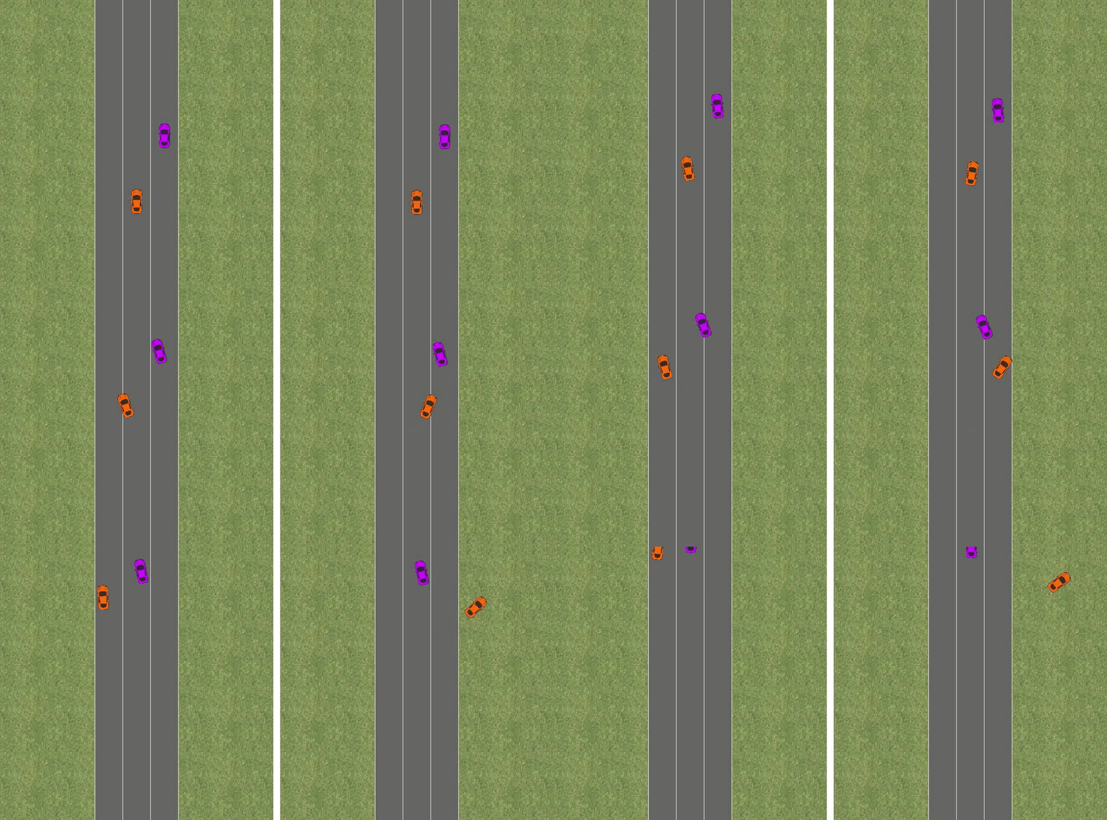
Preference queries: Given the movements of the pink car, which trajectory of the orange car would you prefer following?
In fact, psychologists studied this subject decades ago and concluded humans are pretty reliable on answering preference queries when the number of options to compare is low enough$^1$. In this post, we will focus on pairwise comparisons. Given we can now reliably collect data, the next natural question would be: How are we going to use these comparisons to learn the underlying reward function?
To develop our learning algorithm, we will first model the structure of the reward function. We will assume that the reward value of a trajectory is a linear function of some high-level features:
\[R(\xi) = \omega^T\phi(\xi)\]For example, for an autonomous driving task, these features could be the alignment of the car with the road and with the lane, the speed, the distance to the closest car, etc$^2$. In this autonomous driving context, $\xi$ represents a trajectory, $\phi(\xi)$ is the corresponding feature-vector and $\omega$ is a vector consisting of weights that define the reward function.
We then model how humans make their choices, again based on some psychology literature$^3$. Given two trajectories $\xi_A$ and $\xi_B$, the difference on the reward values is simply $\omega^T(\phi(\xi_A)-\phi(\xi_B)) = \omega^T\psi$. Then, the probability of user choosing $\xi_A$ is:
\[P(I_A | \omega) = \frac{1}{1+\exp(-I_A\omega^T\psi)}\]where $I_A = \textrm{sign}(\omega^T\psi)$, and it being either 1 or -1 shows the output of the query.

The model of the overall decision process. The dynamical system denoted by $\mathcal{D}$ produces the trajectories with respect to its initial state $x_0$ and control inputs of human and robot agents $u_H$ and $u_R$. The output of the query is then a linear combination of the difference in the trajectory features.
The way we are going to learn the weights vector, and by extension the reward function, is Bayesian: $p(\omega \mid I_i) \propto p(I_i \mid \omega) p(\omega)$, where $i$ denotes the query number, and after each query we update the distribution over $\omega$.
Up to this point, we have shown how preference-based learning can help in robot learning. However, there remains an important problem: How many such comparisons are needed to have the robot learn the reward function? And is it always possible to learn the reward function in this way?
Active Preference-based Learning
To reduce the number of required comparisons, we want to actively synthesize queries, i.e. we want to maximize the information received from each query to learn the reward function as quickly as possible. While optimal querying is NP-hard, Sadigh et al. showed that modeling this problem as a maximum volume removal problem works well in practice (see this paper). In the same work, they also showed the query selection problem can be formulated as:
\[\max_{x^0, {u_H}_A, {u_H}_B, u_R} \min\{E[1-p(I_i \mid \omega)], E[1-p(-I_i \mid \omega)]\}\]where the robot actions and the initial state are assumed to be identical among the two query trajectories. The optimization objective can be approximated by sampling $\omega$ and the optimization can be locally solved. One can easily note that we want to generate the queries for which we are very unsure about the outcome with the current knowledge of $\omega$. Another interpretation is that we want to maximize the conditional entropy of Ii given $\omega$. While the practicality of this method has been analyzed in this paper, query generation times remained a huge limitation.
Batch-Active Preference-based Learning
To speed up the query synthesization process, we can generate a batch of queries at once. This is again NP-hard to do optimally. Moreover, the queries to be generated are not independent. One query might carry a significant portion of information that another query already has. In this case, while both queries are individually very informative, having both of them in the batch is wasteful.
Then, we can describe the problem as follows. We have one feature difference vector $\psi$ for each query. And for each of them, we can compute the optimization objective given above. While these values will represent how much we desire that query to be in the batch, we also want $\psi$-values to be as different as possible from each other.
The general approach to this problem is the following: Among $M$ queries, we first select $B$ of them that individually maximize the optimization objective. To further select $b$ queries from this preselected set to eliminate similarities between queries, we present four different methods:
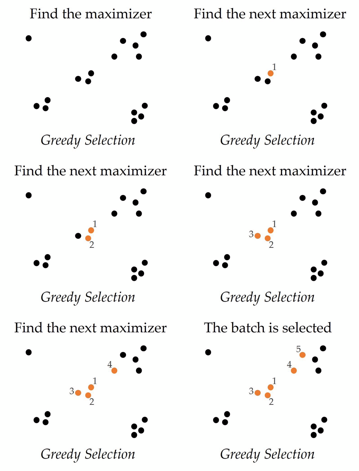
- Greedy Selection: We simply select $b$ individual maximizers.
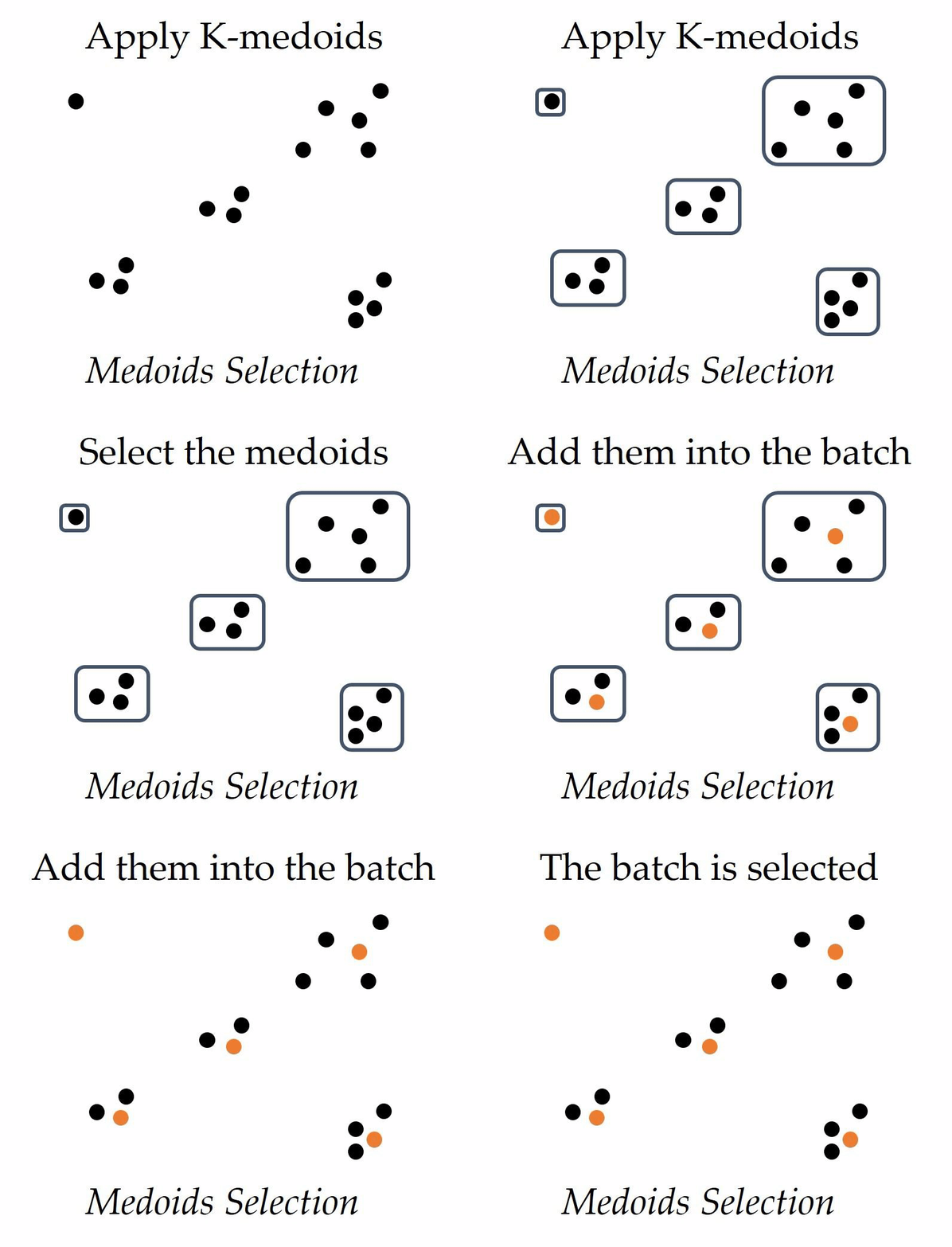
- Medoids Selection: We cluster $\psi$-vectors using K-medoids algorithm into $b$ clusters and then we select the medoids.
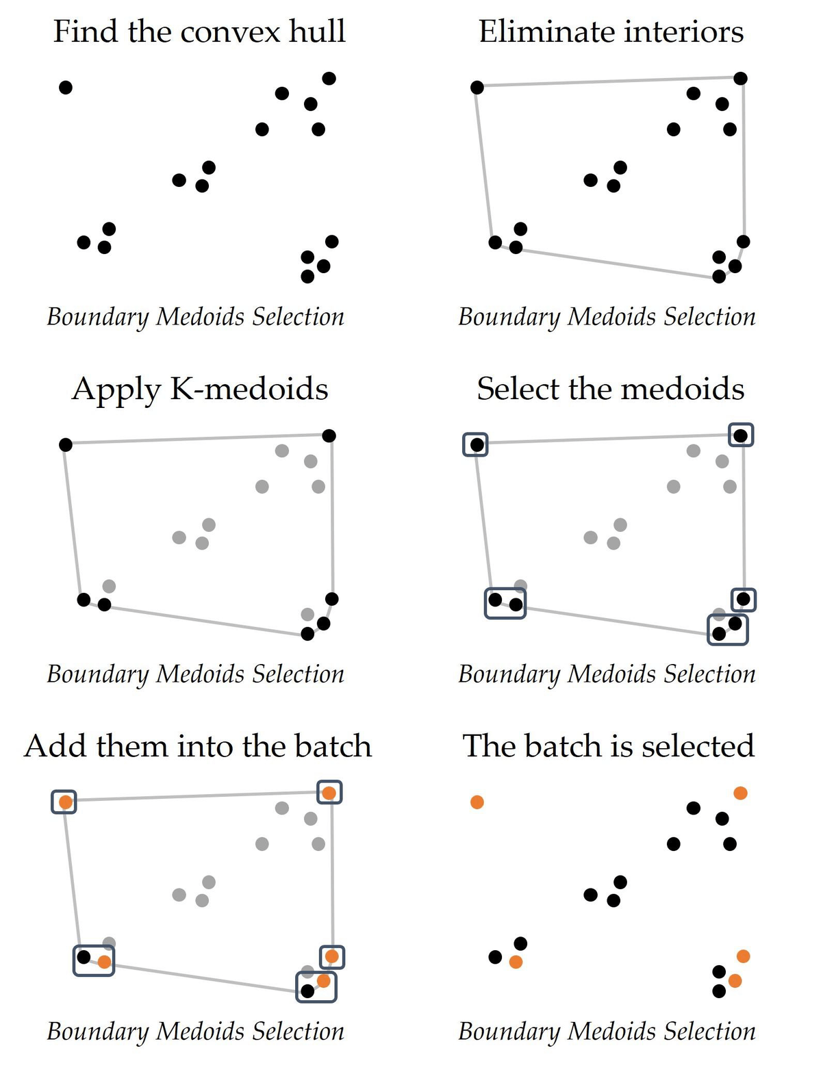
- Boundary Medoids Selection: Medoids selection algorithm can be improved by only choosing the queries that correspond to the boundary. For that, we first take the convex hull of the preselected set and eliminate the queries that are inside this volume. Then, we apply K-medoids algorithm on the remaining vectors to cluster them into $b$ clusters, and then finally we select the medoids.
- Successive Elimination: An important observation is that the problem we are trying to solve while selecting $b$ of the queries out of the preselected set is actually similar to the max-sum diversification problem, where the aim is to select a fixed-size subset of points whose average distance to each other is maximized. Unfortunately, this problem is also known to be NP-hard. However, our problem is slightly different, because we have the optimization objective values that represent the value of each query to us. Hence, we propose the following algorithm: At every iteration of the algorithm, we select two closest points in the preselected set, and remove the one with lower information entropy (or optimization objective). And we repeat this until we end up with $b$ queries.
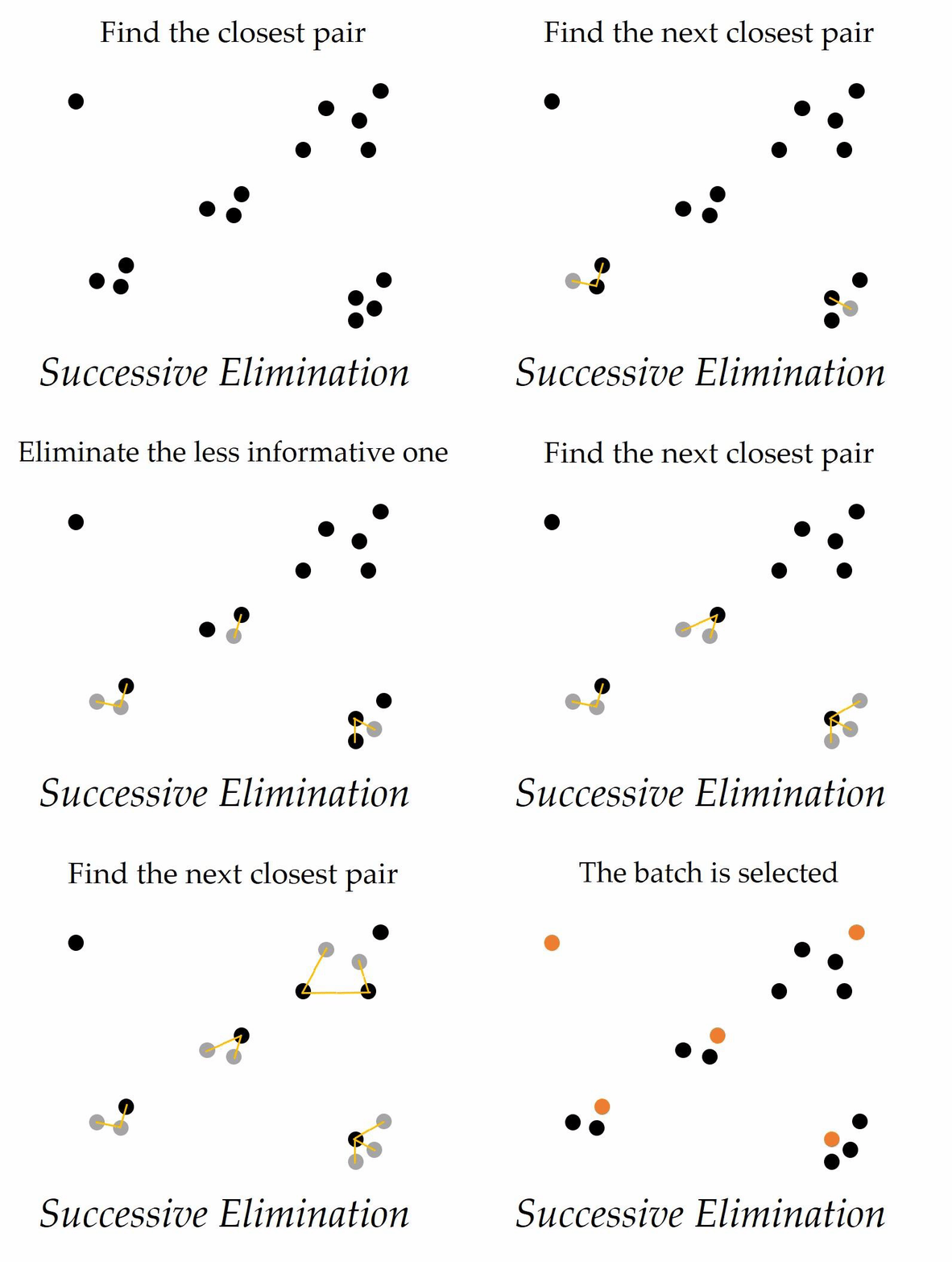
Theoretical Guarantees: In the paper, we have showed the convergence is guaranteed under some additional assumptions with greedy selection and successive elimination methods, as they will always keep the most informative query in the batch.
Experiments & Results
We did experiments with a simple linear dynamical system (LDS) and 5 different simulations from MuJoCo, OpenAI Gym, and a driving simulator presented in another work. We assumed a true reward function and attempted to estimate it using our methods with $b=10$.

Views from each simulated task.
We evaluated each algorithm with a metric $m$ that quantifies how close the estimated reward function is to the true function after $N$ queries. So, how well did the various querying methods do?
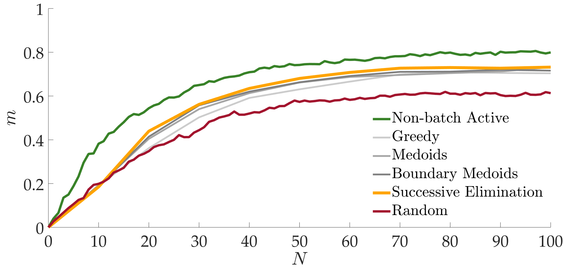
There we have it: the greedy algorithm is significantly outperformed by the three other batch-active methods. The performances are ordered from the worst to the best as greedy, medoids, boundary medoids, and successive elimination. In fact successive elimination significantly outperformed medoid selection, too.
Simulated environments also led to similar results and showed the time-efficiency of batch-active methods. They also showed how local optima can potentially impair the non-batch active method.
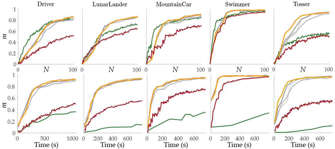
In the table below, we show the average query time in seconds for each method.
| Task Name | Non-Batch | Batch-Active Learning Methods | |||
|---|---|---|---|---|---|
| Greedy | Medoids | Boundary Medoids | Successive Elimination | ||
| Driver | 79.2 | 5.4 | 5.7 | 5.3 | 5.5 |
| LunarLander | 177.4 | 4.1 | 4.1 | 4.2 | 4.1 |
| MountainCar | 96.4 | 3.8 | 4.0 | 4.0 | 3.8 |
| Swimmer | 188.9 | 3.8 | 3.9 | 4.0 | 4.1 |
| Tosser | 149.3 | 4.1 | 4.3 | 3.8 | 3.9 |
Batch active results in a speed up of factor 15 to 50 ! As one might infer there is a tradeoff between how fast we generate queries and how fast we converge to the true reward function in terms of the number of queries.
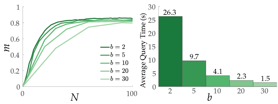
Lastly, we perform usability studies by recruiting 10 human subjects to respond the queries for Driver and Tosser tasks. We have seen that our methods are able to efficiently learn different human preferences.
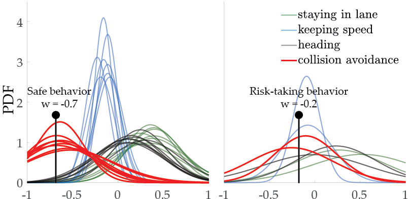
The distributions of weights for 10 different people on the Driver task.

The distributions of weights for 10 different people on the Tosser task.
We also present demonstrative examples of the learning process for both simulation environments.
Driver: https://www.youtube.com/watch?v=MaswyWRep5g
Tosser: https://www.youtube.com/watch?v=cQ7vvUg9rU4
What’s Next?
So, as our results showed Batch Active learning not only improves convergence but does it fast. We are very enthusiastic about the continuation of this work. Some potential directions that we are currently working on include, but are not limited to:
- Varying batch-sizes could increase performance, i.e. it is intuitively a good idea to start with small batches and then increase batch size as we start with no information.
- To improve the usability in complex tasks, an end-to-end framework that also learns the feature transformations would help a lot.
- While the current approach is useful with simulations, it is important to incorporate safety constraints when working with actual robots. In other words, we cannot simply generate trajectories with any input when the system of interest is safety-critical. Hopefully, an extension of this work will one day make machine learning as successful in robotics as in the other domains where it already works wonders.
$^1$ See, for example, this famous paper.
$^2$ This assumption is actually pretty mild, because those high-level feature transformations of trajectories could be the neural network embeddings.
$^3$ See Luce’s choice axiom and this work.
This post is based on the following paper:
Batch Active Preference-Based Learning of Reward Functions (arXiv)
Erdem Bıyık, Dorsa Sadigh
Proceedings of the 2nd Conference on Robot Learning (CoRL), October 2018
